Optimization of a State-to-State Transfer in a Two-Level-System
$\gdef\op#1{\hat{#1}}$ $\gdef\init{\text{init}}$ $\gdef\tgt{\text{tgt}}$
This first example illustrates the basic use of the GRAPE.jl by solving a simple canonical optimization problem: the transfer of population in a two level system.
datadir(names...) = joinpath(@__DIR__, names...)

using QuantumControl
using QuantumPropagators: ExpProp
Two-level Hamiltonian
We consider the Hamiltonian $\op{H}_{0} = - \frac{\omega}{2} \op{\sigma}_{z}$, representing a simple qubit with energy level splitting $\omega$ in the basis $\{\ket{0},\ket{1}\}$. The control field $\epsilon(t)$ is assumed to couple via the Hamiltonian $\op{H}_{1}(t) = \epsilon(t) \op{\sigma}_{x}$ to the qubit, i.e., the control field effectively drives transitions between both qubit states.
ϵ(t) = 0.2 * QuantumControl.Shapes.flattop(t, T=5, t_rise=0.3, func=:blackman);"""Two-level-system Hamiltonian."""
function tls_hamiltonian(Ω=1.0, ϵ=ϵ)
σ̂_z = ComplexF64[
1 0
0 -1
]
σ̂_x = ComplexF64[
0 1
1 0
]
Ĥ₀ = -0.5 * Ω * σ̂_z
Ĥ₁ = σ̂_x
return hamiltonian(Ĥ₀, (Ĥ₁, ϵ))
end;H = tls_hamiltonian();The control field here switches on from zero at $t=0$ to it's maximum amplitude 0.2 within the time period 0.3 (the switch-on shape is half a Blackman pulse). It switches off again in the time period 0.3 before the final time $T=5$). We use a time grid with 500 time steps between 0 and $T$:
tlist = collect(range(0, 5, length=500));using Plots
Plots.default(
linewidth = 3,
size = (550, 300),
legend = :right,
foreground_color_legend = nothing,
background_color_legend = RGBA(1, 1, 1, 0.8)
)function plot_control(pulse::Vector, tlist)
plot(tlist, pulse, xlabel="time", ylabel="amplitude", legend=false)
end
plot_control(ϵ::Function, tlist) = plot_control([ϵ(t) for t in tlist], tlist);fig = plot_control(ϵ, tlist)
Optimization target
First, we define a convenience function for the eigenstates.
function ket(label)
    result = Dict("0" => Vector{ComplexF64}([1, 0]), "1" => Vector{ComplexF64}([0, 1]))
    return result[string(label)]
end;
The physical objective of our optimization is to transform the initial state $\ket{0}$ into the target state $\ket{1}$ under the time evolution induced by the Hamiltonian $\op{H}(t)$.
trajectories = [Trajectory(initial_state=ket(0), generator=H, target_state=ket(1))];The full control problem includes this trajectory, information about the time grid for the dynamics, and the functional to be used (the square modulus of the overlap $\tau$ with the target state in this case).
using QuantumControl.Functionals: J_T_sm

problem = ControlProblem(
    trajectories=trajectories,
    tlist=tlist,
    iter_stop=500,
    prop_method=ExpProp,
    pulse_options=Dict(),
    J_T=J_T_sm,
    check_convergence=res -> begin
        ((res.J_T < 1e-3) && (res.converged = true) && (res.message = "J_T < 10⁻³"))
    end,
);
Simulate dynamics under the guess field
Before running the optimization procedure, we first simulate the dynamics under the guess field $\epsilon_{0}(t)$. The following solves equation of motion for the defined trajectory, which contains the initial state $\ket{\Psi_{\init}}$ and the Hamiltonian $\op{H}(t)$ defining its evolution.
guess_dynamics = propagate_trajectory(
    trajectories[1],
    problem.tlist;
    method=ExpProp,
    storage=true,
    observables=(Ψ -> abs.(Ψ) .^ 2,)
)
2×500 Matrix{Float64}:
1.0 1.0 1.0 1.0 … 0.951457 0.951459 0.951459
0.0 7.73456e-40 2.03206e-11 2.96638e-10 0.0485427 0.048541 0.048541function plot_population(pop0::Vector, pop1::Vector, tlist)
fig = plot(tlist, pop0, label="0", xlabel="time", ylabel="population")
plot!(fig, tlist, pop1; label="1")
end;fig = plot_population(guess_dynamics[1, :], guess_dynamics[2, :], tlist)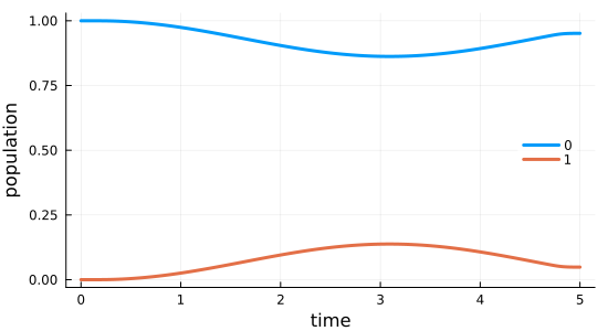
Optimization with LBFGSB
In the following we optimize the guess field $\epsilon_{0}(t)$ such that the intended state-to-state transfer $\ket{\Psi_{\init}} \rightarrow \ket{\Psi_{\tgt}}$ is solved.
The GRAPE package performs the optimization by calculating the gradient of $J_T$ with respect to the values of the control field at each point in time. This gradient is then fed into a backend solver that calculates an appropriate update based on that gradient.
using GRAPEBy default, this backend is LBFGSB.jl, a wrapper around the true and tested L-BFGS-B Fortran library. L-BFGS-B is a pseudo-Hessian method: it efficiently estimates the second-order Hessian from the gradient information. The search direction determined from that Hessian dramatically improves convergence compared to using the gradient directly as a search direction. The L-BFGS-B method performs its own linesearch to determine how far to go in the search direction.
opt_result_LBFGSB = @optimize_or_load(
    datadir("TLS", "GRAPE_opt_result_LBFGSB.jld2"),
    problem;
    method=GRAPE,
    prop_method=ExpProp,
);
[ Info: Set callback to store result in TLS/GRAPE_opt_result_LBFGSB.jld2 on unexpected exit.
iter. J_T ǁ∇Jǁ ǁΔϵǁ ΔJ FG(F) secs
0 9.51e-01 5.40e-02 n/a n/a 1(0) 1.4
1 9.49e-01 5.40e-02 5.40e-02 -2.95e-03 1(0) 0.2
2 3.94e-02 5.55e-02 9.54e+00 -9.09e-01 6(0) 0.0
3 1.65e-02 6.30e-02 1.34e+00 -2.29e-02 2(0) 0.0
4 1.27e-02 3.82e-02 1.64e+00 -3.84e-03 1(0) 0.0
5 1.65e-05 3.35e-02 7.42e-01 -1.27e-02 1(0) 0.0
opt_result_LBFGSBGRAPE Optimization Result
-------------------------
- Started at 2024-12-02T17:24:43.961
- Number of trajectories: 1
- Number of iterations: 5
- Number of pure func evals: 0
- Number of func/grad evals: 12
- Value of functional: 1.65005e-05
- Reason for termination: J_T < 10⁻³
- Ended at 2024-12-02T17:24:45.633 (1 second, 672 milliseconds)
We can plot the optimized field:
fig = plot_control(opt_result_LBFGSB.optimized_controls[1], tlist) # This is test
Optimization via semi-automatic differentiation
Our GRAPE implementation includes the analytic gradient of the optimization functional J_T_sm. Thus, we only had to pass the functional itself to the optimization. More generally, for functionals where the analytic gradient is not known, semi-automatic differentiation can be used to determine it automatically. For illustration, we may re-run the optimization forgoing the known analytic gradient and instead using an automatically determined gradient.
As shown in Goerz et al., arXiv:2205.15044, by evaluating the gradient of $J_T$ via a chain rule in the propagated states, the dependency of the gradient on the final time functional is pushed into the boundary condition for the backward propagation, $|χ_k⟩ = -∂J_T/∂⟨ϕ_k|$. For functionals that can be written in terms of the overlaps $τ_k$ of the forward-propagated states and target states, such as the J_T_sm used here, a further chain rule leaves derivatives of J_T with respect to the overlaps $τ_k$, which are easily obtained via automatic differentiation. The optimize function takes an optional parameter chi that may be passed a function to calculate $|χ_k⟩$. A suitable function can be obtained using
using QuantumControl.Functionals: make_chiTo force make_chi to use automatic differentiation, we must first load a suitable AD framework
using ZygoteThen, we can pass mode=:automatic and automatic=Zygote to make_chi:
chi_sm = make_chi(J_T_sm, trajectories; mode=:automatic, automatic=Zygote)(::QuantumControlZygoteExt.var"#zygote_chi_via_tau#6"{QuantumControlZygoteExt.var"#zygote_chi_via_tau#2#7"{typeof(QuantumControl.Functionals.J_T_sm)}}) (generic function with 1 method)The resulting chi_sm can be used in the optimization:
opt_result_LBFGSB_via_χ = optimize(problem; method=GRAPE, chi=chi_sm); iter. J_T ǁ∇Jǁ ǁΔϵǁ ΔJ FG(F) secs
0 9.51e-01 5.40e-02 n/a n/a 1(0) 8.3
1 9.49e-01 5.40e-02 5.40e-02 -2.95e-03 1(0) 0.1
2 3.94e-02 5.55e-02 9.54e+00 -9.09e-01 6(0) 0.0
3 1.65e-02 6.30e-02 1.34e+00 -2.29e-02 2(0) 0.0
4 1.27e-02 3.82e-02 1.64e+00 -3.84e-03 1(0) 0.0
5 1.65e-05 3.35e-02 7.42e-01 -1.27e-02 1(0) 0.0
opt_result_LBFGSB_via_χGRAPE Optimization Result
-------------------------
- Started at 2024-12-02T17:25:10.892
- Number of trajectories: 1
- Number of iterations: 5
- Number of pure func evals: 0
- Number of func/grad evals: 12
- Value of functional: 1.65005e-05
- Reason for termination: J_T < 10⁻³
- Ended at 2024-12-02T17:25:19.318 (8 seconds, 426 milliseconds)
Optimization with Optim.jl
As an alternative to the default L-BFGS-B backend, we can also use any of the gradient-based optimizers in Optim.jl. This also gives full control over the linesearch method.
import Optim
import LineSearches
Here, we use the LBFGS implementation that is part of Optim (which is not exactly the same as L-BFGS-B; "B" being the variant of LBFGS with optional additional bounds on the control) with a Hager-Zhang linesearch
opt_result_OptimLBFGS = @optimize_or_load(
    datadir("TLS", "GRAPE_opt_result_OptimLBFGS.jld2"),
    problem;
    method=GRAPE,
    optimizer=Optim.LBFGS(;
        alphaguess=LineSearches.InitialStatic(alpha=0.2),
        linesearch=LineSearches.HagerZhang(alphamax=2.0)
    ),
);
[ Info: Set callback to store result in TLS/GRAPE_opt_result_OptimLBFGS.jld2 on unexpected exit.
1 9.51e-01 0.00e+00 0.00e+00 9.51e-01 1(0) 1.0
2 9.45e-01 5.40e-02 1.08e-01 -5.99e-03 3(0) 0.1
3 9.39e-01 5.71e-02 1.14e-01 -6.72e-03 3(0) 0.0
4 9.31e-01 6.04e-02 1.21e-01 -7.52e-03 3(0) 0.0
5 9.23e-01 6.39e-02 1.28e-01 -8.41e-03 3(0) 0.0
6 9.13e-01 6.76e-02 1.35e-01 -9.39e-03 3(0) 0.0
7 9.03e-01 7.14e-02 1.43e-01 -1.05e-02 3(0) 0.0
8 8.91e-01 7.53e-02 1.51e-01 -1.16e-02 3(0) 0.0
9 8.78e-01 7.94e-02 1.59e-01 -1.29e-02 3(0) 0.0
10 8.64e-01 8.35e-02 1.67e-01 -1.43e-02 3(0) 0.0
11 8.48e-01 8.78e-02 1.76e-01 -1.58e-02 3(0) 0.0
12 8.31e-01 9.22e-02 1.84e-01 -1.74e-02 3(0) 0.1
13 8.12e-01 9.66e-02 1.93e-01 -1.91e-02 3(0) 0.0
14 7.91e-01 1.01e-01 2.02e-01 -2.08e-02 3(0) 0.0
15 7.68e-01 1.05e-01 2.11e-01 -2.26e-02 3(0) 0.0
16 7.44e-01 1.10e-01 2.19e-01 -2.45e-02 3(0) 0.0
17 7.18e-01 1.14e-01 2.27e-01 -2.63e-02 3(0) 0.0
18 6.90e-01 1.17e-01 2.35e-01 -2.80e-02 3(0) 0.0
19 6.60e-01 1.21e-01 2.42e-01 -2.97e-02 3(0) 0.0
20 6.29e-01 1.24e-01 2.49e-01 -3.12e-02 3(0) 0.0
21 5.96e-01 1.27e-01 2.54e-01 -3.26e-02 3(0) 0.0
22 5.62e-01 1.29e-01 2.59e-01 -3.37e-02 3(0) 0.0
23 5.28e-01 1.31e-01 2.62e-01 -3.45e-02 3(0) 0.0
24 4.93e-01 1.32e-01 2.64e-01 -3.50e-02 3(0) 0.0
25 4.58e-01 1.33e-01 2.65e-01 -3.51e-02 3(0) 0.0
26 7.25e-02 1.32e-01 5.28e+01 -3.85e-01 2(0) 0.0
27 1.68e-02 4.32e-02 2.54e+00 -5.57e-02 2(0) 0.0
28 2.50e-05 4.51e-02 1.11e+00 -1.68e-02 3(0) 0.0
opt_result_OptimLBFGSGRAPE Optimization Result
-------------------------
- Started at 2024-12-02T17:24:57.333
- Number of trajectories: 1
- Number of iterations: 28
- Number of pure func evals: 0
- Number of func/grad evals: 80
- Value of functional: 2.49647e-05
- Reason for termination: J_T < 10⁻³
- Ended at 2024-12-02T17:24:58.990 (1 second, 657 milliseconds)
We can plot the optimized field:
fig = plot_control(opt_result_OptimLBFGS.optimized_controls[1], tlist)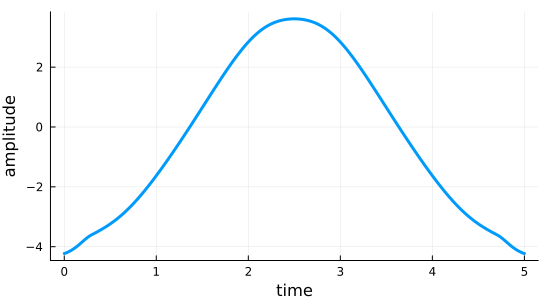
We can see that the choice of linesearch parameters in particular strongly influence the convergence and the resulting field. Play around with different methods and parameters!
Empirically, we find the default L-BFGS-B to have a very well-behaved linesearch.
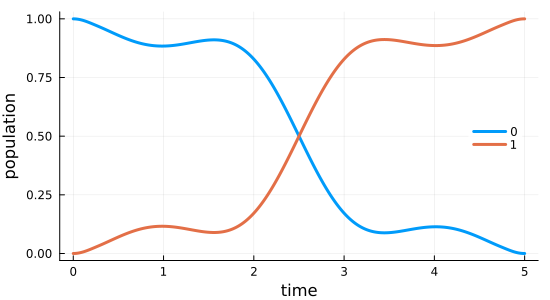
Simulate the dynamics under the optimized field
Having obtained the optimized control field, we can simulate the dynamics to verify that the optimized field indeed drives the initial state $\ket{\Psi_{\init}} = \ket{0}$ to the desired target state $\ket{\Psi_{\tgt}} = \ket{1}$.
using QuantumControl.Controls: substitute

opt_dynamics = propagate_trajectory(
    substitute(trajectories[1], IdDict(ϵ => opt_result_LBFGSB.optimized_controls[1])),
    problem.tlist;
    method=ExpProp,
    storage=true,
    observables=(Ψ -> abs.(Ψ) .^ 2,)
)
2×500 Matrix{Float64}:
1.0 0.99994 0.999762 … 0.000174609 3.65549e-5 1.65005e-5
0.0 5.96719e-5 0.000237653 0.999825 0.999963 0.999983fig = plot_population(opt_dynamics[1, :], opt_dynamics[2, :], tlist)